Iso-surface of 15% deficit enclosing the wake tubereplace with screenshot · 1200 × 750
Add an iso-surface node on the deficit field and set the threshold to 0.15. A ghostly tube appears behind the rotor in the 3D viewer, showing exactly where the wake has and hasn't recovered. Drag the threshold slider to tighten or loosen the envelope — the mesh rebuilds live from the cached field.
Inputs
deficit — the derived velocity-deficit field to contour
Parameters
threshold — deficit level the iso-surface encloses; drag to tighten or loosen the envelope0.15
Outputs
wake mesh — iso-surface tube enclosing the unrecovered wake behind the rotor
Spatial join linking each meter to the building footprint it sits inreplace with screenshot · 1200 × 750
Chain a @shape spatial-join node that drops each meter coordinate into the building footprint it falls inside. The preview draws a line from every meter to its host building so stray gauges stand out. Each reading is now tagged with a building ID.
Inputs
meters — meter coordinates (lat/long) pulled from the meter registry
buildings — building footprints each meter coordinate may fall inside
Parameters
predicate — matches each meter to the footprint its coordinate falls insidewithin
True — meter coordinate used to place it in a building footprintlat/long
Outputs
tagged — each meter reading now tagged with the building ID it sits inside
Bridge mesh rendered around the plotted gauge pointsreplace with screenshot · 1200 × 750
Drop the bridge's glTF export next to it and the structure renders around the floating gauge points. Line the two up and the gauges settle onto the girders and deck where they are actually bonded. Now every reading has a place to land on the geometry.
Parameters
format — Design-model export loaded as the structure geometryglTF
Export node writing styled Shapefile layers and a clean parcel-to-zone CSVreplace with screenshot · 1200 × 750
Style the joined layer with a zone-color palette, then wire a @deliver node that writes styled Shapefile layers plus a clean parcel-to-zone table. Export drops the layers for GIS and a flat CSV the planning team can open in a spreadsheet — parcel ID, zone, and conflict flag, no geometry. When the zoning table updates in PostGIS, re-run and both exports refresh.
Inputs
flagged — The joined, zone-styled parcel layer carrying conflict flags
Parameters
palette — Color palette applied to the joined layer by zonezone-color
csv cols — Columns written to the flat table — parcel ID, zone, flag, no geometryid, zone, flag
Outputs
exports — Styled Shapefile layers plus a flat parcel-to-zone CSV
Scored output preview beside the metrics dashboardreplace with screenshot · 1200 × 750
Point the @deliver export at `scored/` and toggle the report on. You get one scored Parquet file plus a dashboard — score distribution, null counts, rows per second, and drift against the training feature stats.
Inputs
scored — Scored entity carrying the p_convert column
Parameters
path — Output directory the export writes the scored Parquet intoscored/
Campus heat-map colored by live draw beside the weekly report layoutreplace with screenshot · 1200 × 750
Wire the hourly table into a @deliver node that colors each building blue-to-red by current draw — the campus repaints as the feed updates. Add a report delivery set to weekly and it bakes trends, top buildings, and heat-map snapshots into a PDF. Both outputs rebuild from the same canvas.
Inputs
hourly — hourly kWh-per-building table that drives the building colors
Parameters
color — each building colored blue-to-red by its current live drawblue-to-red
schedule — cadence the energy report is baked and delivered onweekly
Outputs
report — weekly energy PDF baking trends, top buildings, and heat-map snapshots
Drift detector with threshold sliders and flagged tagsreplace with screenshot · 1200 × 750
Add the drift detector and set two thresholds with sliders — slope per day for slow drift, jump size for step changes. Flags appear on the chart the moment a tag crosses either one. Tighten a slider and watch borderline sensors flip in and out of the flagged list.
Inputs
baselined — Percent-of-baseline tags coming out of the baseline step
Parameters
drift slope — Slow-drift threshold — a tag flags when its daily slope exceeds thisslope per day
step jump — Step-change threshold — flags an abrupt jump larger than thisjump size
Outputs
flagged tags — Tags that crossed either threshold, marked live on the chart
Motion scores with corrupted slices centered in the viewerreplace with screenshot · 1200 × 750
Add a motion-artifact node that scores each volume for ghosting and ringing. Borderline studies surface for a quick look in the viewer; the obviously corrupted ones light up red on their own. Scrub any flagged study and the offending slices are already centered for you.
Inputs
studies — Cohort studies whose volumes get scored for artifacts
Parameters
artifacts — Artifact types scored on each volumeghosting + ringing
flagging — Borderline studies surface for a viewer look; corrupted ones auto-flag redborderline + red
Outputs
scores — Per-study motion score with offending slices already centered in the viewer
3D flyover of the flood-risk raster draped over the valley terrainreplace with screenshot · 1200 × 750
Wire the risk grid into the 3D viewer and drape it over the LiDAR terrain. Scrub the camera down each valley to see which streets and parcels sit inside the 100-year footprint, and toggle return periods to compare scenarios in place. When a stakeholder asks about one block, you fly straight to it instead of re-rendering.
Inputs
risk — Flood-risk raster to drape over the terrain
terrain — LiDAR terrain surface for the 3D scene
Parameters
drape — Drape the risk raster over the terrain surfaceon
return — Toggle return periods to compare scenarios in place10-100 yr
Outputs
flyover — Scrubbable 3D scene you fly down each valley
Export node with GeoTIFF and glTF outputs configuredreplace with screenshot · 1200 × 750
Wire the grid into a @deliver node set to GeoTIFF and send the fused cloud out as glTF for the sim team. Hit export and both files land in the nav stack's map folder. When new sweeps arrive, the same canvas rebuilds both exports untouched.
Inputs
grid — the baked 2D occupancy grid for the nav stack
fused cloud — the registered 3D cloud for the sim team
Parameters
grid fmt — raster format for the 2D occupancy gridGeoTIFF
cloud fmt — mesh format for the fused 3D cloudglTF
Outputs
map files — GeoTIFF + glTF written to the nav stack's map folder
Baselined tags plotted as percent deviation from Mondayreplace with screenshot · 1200 × 750
Chain a baseline step that takes each tag's Monday median as its reference and rescales the week to percent-of-baseline. Sensors with different units and ranges become directly comparable. Flat lines mean healthy; anything sloping is a suspect.
Inputs
tags — Resampled sensor tags aligned on the shared 1-minute time base
Parameters
reference — Each tag's Monday median taken as its baseline referenceMonday median
rescale — Week rescaled to percent-of-baseline so mixed units compare directly% of baseline
Outputs
pct-baseline — Each tag rescaled to percent of its own Monday reference
200 ragged series resampled onto one aligned one-minute gridreplace with screenshot · 1200 × 750
Chain a sync node and pick a one-minute common grid. Set interpolation for the analog channels and hold-last for the slow ones, and watch 200 ragged timelines snap into one aligned table. That aligned table is a cached intermediate, so every statistic downstream recomputes instantly.
Inputs
series — 200 per-sensor time series with ragged, unaligned timestamps.
Parameters
grid — Common time step every sensor is resampled onto.1 min
analog — Fill method for fast analog channels between samples.interpolate
slow chans — Fill method for slow channels — carry the last reading forward.hold-last
Outputs
aligned table — All 200 sensors resampled onto one shared clock; cached intermediate.
Log bundle grouped by unit with type-inferred previewsreplace with screenshot · 1200 × 750
Drag the trial folder — 12 units, six sensor CSVs each — onto the canvas. LSD groups them into one @load node keyed by unit ID and previews the first rows with inferred types. IMU at 200 Hz, GPS at 5 Hz, and battery at 1 Hz land as separate time-series entities.
Parameters
key — Column the trial folder is grouped by, one entity per robotunit ID
types — Column types auto-detected from the first rows of each CSVinferred
Outputs
series — Per-unit IMU/GPS/battery time-series entities grouped by unit ID
preview — First rows of each CSV with inferred column types
Organ labels streaming in over the axial slicesreplace with screenshot · 1200 × 750
Drop your ONNX organ model onto the canvas and wire the resampled volume into the @deliver node it becomes. Labels stream back a slice block at a time, and the viewer paints each organ its own color as they arrive. A flipped orientation or wrong label index shows up in seconds — long before the full volume finishes.
Inputs
iso volume — Resampled isotropic CT volume fed into the ONNX model
Parameters
model — The ONNX organ segmentation model executed on the volumeONNX
Outputs
labels — Per-organ label volume streamed back a slice block at a time
Timeline painted with red dropout bands and amber outlier flagsreplace with screenshot · 1200 × 750
Add two flag nodes — a rolling MAD outlier check on every numeric channel, and a gap detector that marks any silence over 500 ms as a dropout. Flags paint straight onto the timeline as red and amber bands. Unit 7's IMU lights up immediately with forty dropouts an hour.
Inputs
synced — Merged 10 Hz timeline from the sync node
Parameters
method — Outlier test applied to every numeric channelrolling MAD
gap — Silence longer than this is marked as a dropout500 ms
Outputs
outliers — Amber flags where a channel exceeds the rolling MAD threshold
dropouts — Red bands where a channel goes silent past the gap limit
Twelve Parquet files merging into one snapshot entityreplace with screenshot · 1200 × 750
Drag twelve monthly `snapshot_*.parquet` files onto the canvas together. LSD unions them into one entity, derives a `snapshot_month` column from the filenames, and caches the result — 2.1M account rows with a `churned_within_90d` label.
Parameters
files — twelve monthly snapshot_*.parquet files unioned into one entity12 × parquet
month_col — column derived from each source filenamesnapshot_month
Outputs
snapshots — 2.1M account rows, one per account per month, carrying the churned_within_90d label
Bridge color-mapped by live stress beside the exported alert logreplace with screenshot · 1200 × 750
Wire the calibrated stress into a @deliver node that colors the mesh green-to-red by live load — the bridge repaints as each axle rolls across. Set an alert-log delivery that writes every exceedance window to CSV with gauge, time, and peak. Drop a new telemetry batch and both rebuild from cached intermediates.
Inputs
stress — Calibrated live stress that drives the green-to-red mesh color
exceedance — Flagged windows where a gauge crossed its limit, for the alert log
Parameters
colorramp — Mesh color scale mapped low-to-high by live stressgreen-to-red
log-fmt — Alert-log export format with one row per exceedance windowCSV
Outputs
alert-log — CSV row per exceedance window with gauge, time, and peak stress
Per-run dark subtraction and flat division previewing livereplace with screenshot · 1200 × 750
Add a @shape node that subtracts the matched dark frame and divides by the flat-field response for every run. The corrected preview updates live as you choose which dark to pair by exposure time. The full corrected stack becomes a cached intermediate, so every step after it stays instant.
Inputs
runs — raw per-run spectra grouped from the CSV folder
calib — dark frames and flat-field response from the calibration NetCDF
Parameters
pair by — matches each run to its dark frame by exposure timeexposure time
correct — subtract matched dark then divide by flat-field responsedark & flat
Outputs
corrected — dark-subtracted, flat-divided stack cached as an intermediate
Per-unit pass/fail report with threshold breakdownreplace with screenshot · 1200 × 750
Finish with a @deliver report node and set the trial thresholds — dropouts under 0.5%, outliers under 1%, live heartbeat present. Every unit gets a pass/fail badge with its flagged windows attached as evidence. Export as CSV and post it before anyone loads the truck.
Inputs
flags — Per-unit outlier and dropout flags from the flag nodes
live — Live heartbeat presence per unit from the fleet API
Parameters
dropout — Max dropout fraction a unit may have and still pass< 0.5%
outlier — Max outlier fraction a unit may have and still pass< 1%
Outputs
report.csv — Per-unit pass/fail report with flagged windows attached as evidence
200 sensor logs grouped into one entity with per-sensor row countsreplace with screenshot · 1200 × 750
Drag the archive of long-run CSVs — 200 sensors, months of samples each — onto the canvas. The @load node groups them into one array entity keyed by sensor ID, infers the timestamp and value columns, and previews row counts per sensor. Files parse lazily, so a multi-gigabyte archive opens at once.
Parameters
key — Column used to group rows into one entity per sensor.sensor ID
columns — Timestamp and value columns, auto-inferred from each file.timestamp + value
Outputs
sensor array — One array entity keyed by sensor ID, grouping all 200 sensors' logs.
row counts — Per-sensor row-count preview so short or missing logs stand out.
Hub-height slice plane dragged through the wake in the 3D viewerreplace with screenshot · 1200 × 750
Add a slice node and drag the plane through the domain in the 3D viewer. Snap it to hub height, then add a second vertical plane down the rotor axis. Both previews update as you drag — the full-resolution volume stays on disk as a cached intermediate.
Inputs
volume — the full-resolution CFD field to cut planes through
Parameters
hub plane — elevation the first horizontal slice plane snaps tohub height
axis plane — orientation of the second vertical plane down the rotor axisrotor axis
Outputs
hub slice — horizontal plane snapped to hub height
axis slice — vertical plane running down the rotor axis
The too-clean histogram, before and after re-anchoringreplace with screenshot · 1200 × 750
Sort the feature preview by correlation with the label and `days_since_last_login` glows at 0.96, its histogram split into two clean islands. Click the node and the cause is right there in the expression — the window was anchored to the export date, not the snapshot date. Re-anchor it and the histogram relaxes into honest overlap.
Inputs
features — windowed feature table, sortable by correlation with the churn label
Parameters
anchor — window anchor; changed from export_date so the feature can't see the futuresnapshot_date
corr — correlation with the churn label that exposed the leaky feature before training0.96
Outputs
recency — the re-anchored days_since_last_login feature, now with honest overlap
Class predictions streaming in over the orthomosaicreplace with screenshot · 1200 × 750
Drop the ONNX U-Net onto the canvas and wire the normalized tiles into the @deliver node it becomes. Predictions stream back a batch at a time, and the viewer paints class colors over the imagery as they arrive — a wrong class index shows up in seconds, not after the full run.
Inputs
tiles — Normalized reflectance tiles wired into the ONNX segmentation model
Parameters
model — The ONNX U-Net segmentation model dropped onto the canvasONNX U-Net
stream — Predictions return one batch at a time so a wrong class index shows in secondsper batch
Outputs
predictions — Per-tile class masks streamed back a batch at a time
Time-axis scrubber looping one rotor revolutionreplace with screenshot · 1200 × 750
Scrub the time axis and the slices, iso-surface, and deficit colors all follow. Set the playback range to the last 400 timesteps — one full rotor revolution — and let the viewer loop it. When the wake meandering reads clearly, queue the animation for export at 1600 × 900.
Inputs
wake mesh — iso-surface and slices driven across the time axis
time axis — axis scrubbed to play the wake evolution over time
Parameters
range — playback window set to the last full rotor revolution400 steps
resolution — output frame size for the rendered animation1600 × 900
Indicator-kriged lithology blocks with a cutaway slicereplace with screenshot · 1200 × 750
Point an indicator-kriging node at the validated intervals and set 10 m blocks with a 150 m search radius. The block model previews with cutaway slices, and nudging the radius re-krigs only the volume — the validated logs stay cached upstream.
Inputs
intervals — Validated drillhole intervals feeding the indicator estimator.
Parameters
block — Edge length of each estimation block in the model grid.10 m
radius — Search radius for neighbouring samples around each block.150 m
method — Indicator kriging estimates a probability per lithology code.indicator
Outputs
block model — Indicator-kriged 3D lithology block volume shown with cutaway slices.
Merged 10 Hz timeline across IMU, GPS, and batteryreplace with screenshot · 1200 × 750
Chain a @shape sync node and pick a 10 Hz common clock. Set linear interpolation for IMU and battery, hold-last for GPS fixes, and watch the merged timeline preview line up. The synced table is a cached intermediate, so the flagging downstream stays instant.
Inputs
logs — Grouped per-unit sensor series from the CSV load node
live — Live REST heartbeat rows arriving under the same schema
Parameters
clock — Common sample rate every channel is resampled onto10 Hz
interp — Interpolation used for IMU and battery numeric channelslinear
gps — GPS fixes carried forward instead of interpolatedhold-last
Outputs
synced — Merged 10 Hz table across IMU, GPS and battery, cached as an intermediate
Color-mapped deviation model exported as glTFreplace with screenshot · 1200 × 750
Add an @deliver node set to glTF. The nominal mesh is baked with a blue-to-red deviation map and exported as one portable file. Anyone can spin it in a browser viewer — no metrology software needed.
Inputs
nominal — Nominal mesh that gets the deviation map baked onto it
deviation — Per-point signed deviations that drive the color map
Parameters
format — Export format — one self-contained glTF fileglTF
colormap — Deviation color ramp baked onto the mesh, blue to redblue→red
Outputs
gltf — Single portable glTF file viewable in any browser
Unit-tagged glTF meshes ready for exportreplace with screenshot · 1200 × 750
Finish with a @deliver node set to glTF and get one 48 MB file with every lithology unit as a tagged, georeferenced mesh. It opens in any glTF viewer — nobody downstream needs geology software installed.
Inputs
block model — The kriged lithology block model to convert into meshes.
Parameters
format — Output container; opens in any glTF viewer without geology software.glTF
tagging — Each lithology unit written as its own georeferenced, tagged mesh.per unit
Outputs
model.gltf — Single 48 MB glTF with every unit as a tagged, georeferenced mesh.
Anomaly expression differencing each member against the baseline climatologyreplace with screenshot · 1200 × 750
Drop the 1991–2020 climatology as a second @load and wire a @shape expression that subtracts it — anomaly = season_mean - baseline. Expose the baseline period as a live parameter. Every member's map recolors around zero the moment you connect the node.
Inputs
season_mean — Seasonal mean field for each member
baseline — 1991-2020 climatology on the same grid
Parameters
expression — The difference expression evaluated per memberseason_mean - baseline
period — Baseline period exposed as a live parameter1991-2020
Outputs
anomaly — season_mean minus baseline, recolored around zero
Boundary-straddling parcels flagged red with the live conflict countreplace with screenshot · 1200 × 750
Add a filter node that flags any parcel intersecting more than one zone — the boundary straddlers the planning team actually cares about. The map lights those lots up in red while clean matches fade back, and the live count tells you exactly how many need review. Drag the overlap tolerance to ignore slivers from imperfect edges.
Inputs
joined — The parcel-to-zone joined layer to scan for conflicts
Parameters
min zones — Flag parcels intersecting more than this many zones2
tolerance — Overlap distance ignored so edge slivers don't count as conflicts0.5 m
Outputs
flagged — Parcels marked where they straddle more than one zone
Cohort tree indexed into a study table with sequence metadatareplace with screenshot · 1200 × 750
Drop the cohort root — 400 studies, mixed scanners and sites — onto the canvas. LSD walks the tree and groups every series into one @load node keyed by study and subject ID, reading tags without decoding pixel data. Four hundred studies index in under a minute, and the preview table lists each one with its sequence, field strength, and acquisition date.
Parameters
key — Grouping key that folds every series into one keyed load nodestudy + subject
read — Reads DICOM tags without decoding pixel data, so 400 studies index in under a minutetags only
Outputs
studies — Cohort of 400 DICOM studies grouped into one node by study and subject ID
study table — Preview row per study with sequence, field strength, and acquisition date
Windowed mean and standard-error band with a live window-length sliderreplace with screenshot · 1200 × 750
Add a windowed-stats node and compute mean, standard deviation, and a standard-error band per sensor over a rolling window. Expose the window length as a live parameter and drag it; every curve and its uncertainty band rebreathe from the cached aligned table. No rerun, no waiting.
Inputs
aligned table — The cached, clock-aligned table from the sync step.
Parameters
window — Rolling window length, exposed as a draggable live parameter.live slider
stats — Statistics computed per window — mean, standard deviation, standard error.mean, sd, SE
Outputs
windowed mean — Rolling per-sensor mean over the chosen window length.
SE band — Standard-error band carried alongside every mean.
Per-study pass/fail table with failing checks listedreplace with screenshot · 1200 × 750
Finish the shaping with a @deliver report node and set the cohort rules — protocol orientation, spacing within tolerance, motion score under threshold, required sequences present. Every study earns a pass/fail badge with its failing checks listed as evidence. The table sorts failures to the top so you see the damage first.
Inputs
flagged — Validated, motion-scored study table for every study
Segmented organs as 3D surfaces with per-organ togglesreplace with screenshot · 1200 × 750
Open the 3D viewer and turn each predicted organ into a shaded surface floating inside the windowed volume. Rotate it to catch the classic failures — a liver that leaks into the ribcage, a kidney with a hole punched through it. Toggle organs on and off and scrub the slice overlay to confirm the surface tracks the boundary on every plane.
Inputs
labels — Per-organ label volume returned by the segmentation model
volume — Windowed CT volume the shaded organ surfaces float inside
Parameters
organs — Which organ surfaces are visible; toggle each one on or offall
Outputs
surfaces — Shaded 3D surface per organ, toggled and inspected in the viewer
63 LAS files merging into one drillhole entityreplace with screenshot · 1200 × 750
Select all 63 LAS files and drop them on the canvas as one @load node. LSD reads each header, aligns the GR, density, and LITH code channels across holes, and previews the merged interval table — 9,400 logged metres in a single entity.
Parameters
files — Number of LAS logs read and merged into a single drillhole entity.63 LAS
channels — Log channels aligned across every hole while merging headers.GR, density, LITH
Outputs
intervals — Merged interval table across 63 holes — 9,400 logged metres in one entity.
Drawdown cone collapsing on the time sliderreplace with screenshot · 1200 × 750
Difference each quarterly surface against the 1998 pre-mining baseline and stack the results into one time-enabled volume. Scrub the time slider in the 3D viewer to watch the drawdown cone relax and the pit lake step toward its spill level.
Inputs
surfaces — Kriged quarterly head surfaces coming from the kriging node
Parameters
baseline — Pre-mining year each quarterly surface is differenced against1998
step — Time step stacked into the volume so the slider advances by quarterquarterly
Outputs
volume — Time-enabled 3D drawdown volume you scrub on the time slider
Tile step preview showing the 1024 px cut gridreplace with screenshot · 1200 × 750
Line-scan frames are 8192 × 2048 — far too big for the model. Add a tile step set to 1024 × 1024 with 128 px overlap; the preview draws the cut grid over a sample frame. The tiled set becomes a cached intermediate, so downstream tweaks never re-cut it.
Inputs
frames — full-size 8192 × 2048 line-scan frames from the load node
Parameters
size — crop dimensions the segmentation model expects1024 × 1024
overlap — overlap between adjacent tiles so seam defects are never cut in half128 px
Outputs
tiles — cached set of model-sized crops cut from every frame
Kriged head surface with variance shadingreplace with screenshot · 1200 × 750
Drop a kriging node on the head table and set a spherical variogram with a 1,200 m range on 250 m cells. LSD grids all 112 quarters in one pass, and the variance map shades the pit's north wall red — that's where the next bore should go.
Inputs
heads — Quarterly water-table head table produced by the head-conversion step
Parameters
model — Variogram model fitted to the head dataspherical
range — Variogram range — distance over which heads stay correlated1,200 m
cell — Output grid cell size for every kriged surface250 m
Outputs
surfaces — Kriged head surface for each of the 112 quarters, in one pass
variance — Variance map shading the pit's north wall where bore coverage is thin
Normalize step with its fitted-params panel openreplace with screenshot · 1200 × 750
Import the @shape normalize step saved from the training pipeline instead of rewriting it. Its fitted means and scales come along as cached params, and the preview shows standardized columns immediately — zero train/serve skew by construction.
Inputs
batch — Raw typed batch to standardize before scoring
Parameters
means — Per-column means imported from the training pipeline, not recomputedtraining-fitted
scales — Per-column scales carried over as cached params for zero train/serve skewtraining-fitted
Outputs
normalized — Columns standardized with the training-fitted means and scales
Publication figure beside the exported NetCDF dataset and pipeline filereplace with screenshot · 1200 × 750
Finish with a @deliver node. Render the stacked spectrum as a publication figure with labelled axes and the uncertainty band, then export the corrected, calibrated dataset as NetCDF alongside it. The pipeline file travels with the export, so a reviewer can rebuild every spectrum from the raw CSVs.
Inputs
spectrum — stacked spectrum with its per-wavelength uncertainty band
dataset — corrected, calibrated per-run dataset to export
Parameters
figure — renders stacked spectrum with labelled axes and uncertainty bandlabelled axes
format — dataset exported as NetCDF with the pipeline file attachedNetCDF
Outputs
export — publication figure, NetCDF dataset, and pipeline file together
Canvas with 412 NetCDF volumes loaded as one entityreplace with screenshot · 1200 × 750
Drag the solver's output folder onto the canvas — 412 NetCDF files, about 200 GB. The @load node reads headers only, so u, v, w, and pressure appear with their dimensions in seconds, and the timesteps stack into a single time axis automatically. Nothing is pulled into memory until a downstream step actually needs it.
Parameters
fields — velocity components and pressure read from each NetCDF fileu, v, w, p
read — reads headers lazily so arrays load only when a downstream step needs themheaders only
Outputs
volume — the stacked CFD field with u, v, w, and pressure on the structured grid
time axis — single time axis formed automatically by stacking all 412 timesteps
Lat/lon crop box dragged over the region across all 40 membersreplace with screenshot · 1200 × 750
Add a @shape crop node and drag a lat/lon box over the region in the map preview, snapping it to the basin you care about. All 40 members crop together and the preview redraws as you drag. The global grid stays on disk as a cached intermediate, so nothing gets copied.
Inputs
ensemble — The 40-member entity from the load node
Parameters
region — Bounding box dragged over the region in the map previewlat/lon box
snap — Snap the box edges to the basin outlinebasin
Outputs
cropped — All 40 members cropped together to the region box
Occupancy grid rendered beneath the 3D cloudreplace with screenshot · 1200 × 750
Drop a rasterize node and set 10 cm cells over a 0.2–1.8 m height band. Points inside the band mark cells occupied; everything scanned but empty becomes free space. The grid renders beneath the 3D cloud so you can check each rack against its footprint.
Inputs
cloud — the thinned, ground-removed obstacle cloud to project down
Parameters
cell — ground resolution of each occupancy grid cell10 cm
band — vertical height slice whose points mark a cell occupied0.2-1.8 m
Strip logs with flagged interval errorsreplace with screenshot · 1200 × 750
Add the interval-check step and LSD flags 41 problems — overlapping intervals, gaps, and codes like GRNT that aren't in the 11-code legend. Fix the mapping in the side panel and watch the strip logs re-render clean, hole by hole.
Inputs
intervals — Joined, desurveyed drillhole interval table to check hole by hole.
NetCDF recharge grid draped over the pit terrainreplace with screenshot · 1200 × 750
Drag the climate model's NetCDF onto the canvas and pick the rch variable from the node's dropdown. The 500 m recharge grid drapes over the terrain in the 3D viewer, and a time chip appears on the node showing 336 monthly slices.
Parameters
variable — NetCDF variable picked from the node's dropdownrch
grid — Native cell size of the regional climate-model recharge grid500 m
Outputs
recharge — 500 m recharge grid with 336 monthly slices, draped over the pit terrain
Drift dashboard beside the ranked maintenance shortlistreplace with screenshot · 1200 × 750
Wire an @deliver dashboard showing every flagged tag with its drift score, plus a CSV export of the maintenance shortlist ranked by severity. Next week, drop the new folder on the same canvas — cached intermediates mean only the new files recompute.
Inputs
flagged tags — Flagged tags with their drift scores from the detector
Parameters
rank by — Shortlist rows sorted by drift severity so worst tags surface firstseverity
recompute — Cached intermediates mean only new files recompute next weekcached
Outputs
shortlist CSV — Maintenance shortlist exported as CSV, ranked by severity
Three-plane preview after resampling to 1 mm isotropic voxelsreplace with screenshot · 1200 × 750
CT slices are usually thicker than they are wide, which skews any 3D measurement. Chain a resample @shape node set to 1 mm isotropic voxels and watch the axial, coronal, and sagittal previews line up to true proportions. The resampled volume caches, so the model step downstream never recomputes it.
Inputs
volume — Windowed CT volume with anisotropic, thicker-than-wide slice spacing
Parameters
voxel — Target voxel size applied equally to all three axes (isotropic)1 mm
Outputs
iso volume — Volume resampled to isotropic voxels so 3D measurements read true
All 80,000 parcel polygons previewed on the canvas, colored by land-use codereplace with screenshot · 1200 × 750
Drag the county parcels Shapefile — all 80,000 polygons — onto the canvas. The @load node reads the geometry and the full attribute table without choking, and the preview draws every lot colored by its current land-use code. The inspector shows the file's CRS so you know exactly what you're reprojecting from.
Parameters
file — The county cadastre Shapefile dropped on the canvascounty_parcels.shp
color by — Attribute used to color every lot in the previewland-use code
Outputs
parcels — All 80,000 parcel polygons with geometry and the full attribute table
Parcels recolored by joined zone code across the countyreplace with screenshot · 1200 × 750
Chain a spatial-join node and set the predicate to intersects, matching each parcel to the zoning polygon it falls in. LSD tags all 80,000 parcels with their zone code in one pass, and the preview recolors the map by zone as the join completes. The joined layer is a cached intermediate the rest of the canvas reuses.
Inputs
parcels — Reprojected 80,000-parcel layer to be tagged with zones
zones — Zoning polygons carrying the zone code to attach
Parameters
predicate — Spatial relationship matching each parcel to its zoning polygonintersects
Outputs
joined — Every parcel tagged with the zone code it falls in
Inference step mid-run with throughput readoutreplace with screenshot · 1200 × 750
Hit run and the inference step streams the entity through ONNX Runtime in 64k-row batches. A progress bar tracks throughput, and scores append as a new `p_convert` column you can preview while the run is still going.
Inputs
entity — Normalized batch streamed row-by-row through ONNX Runtime
model — propensity.onnx session supplying the scoring signature
Parameters
batch — Rows per ONNX Runtime inference batch, tracked by the progress bar64k rows
Outputs
scored — Entity with a new p_convert probability column appended
40-panel small-multiple grid with a shared diverging colorbarreplace with screenshot · 1200 × 750
Add a @deliver map node and set it to facet by member. Forty little anomaly maps tile into one figure with a shared diverging colorbar, so the spread across the ensemble reads at a glance. Nudge the color limits once and every panel follows.
Inputs
anomaly — Per-member seasonal anomaly fields
Parameters
facet — Tile one panel per ensemble membermember
colorbar — Shared diverging color scale across every paneldiverging
Outputs
map grid — 40-panel small-multiple figure with a shared colorbar
Stacked load node with all 38 sweeps and the raw intensity-colored previewreplace with screenshot · 1200 × 750
Drag all 38 .laz files from the robot's scan folder onto the canvas. LSD stacks them into a single @load node and previews the raw cloud — 212 million points, colored by intensity. Open the inspector to confirm each sweep's odometry pose came along for the ride.
Parameters
files — every sweep in the robot's scan folder, stacked into one node38 .laz
color — which channel tints the raw cloud previewintensity
Outputs
raw cloud — 212M-point stacked cloud from all 38 sweeps, colored by intensity
poses — per-sweep odometry pose that rode in with each .laz file
Tile grid preview over farmland imageryreplace with screenshot · 1200 × 750
Add a tile step set to 512 × 512 with 64 px overlap. The preview draws the cut grid over the imagery, and each tile keeps its geotransform so predictions land back in the right place. The tiled set caches, so later re-runs skip straight past it.
Inputs
rasters — The six loaded GeoTIFF orthomosaic tiles to cut into model-sized pieces
Parameters
size — Pixel dimensions of each cut tile fed to the model512 × 512
overlap — Overlap between adjacent tiles, blended later to hide seams64 px
Outputs
tiles — 512 px tiles, each carrying its own geotransform for exact placement
Aisle walls snapping into alignment after ICP refinementreplace with screenshot · 1200 × 750
Add a @shape registration node and feed it the embedded odometry poses. Toggle ICP refinement and watch the doubled-up aisle walls snap into single crisp planes in the preview. The registered cloud is a cached intermediate, so nothing downstream ever re-runs the alignment.
Inputs
raw cloud — the 212M-point stacked cloud straight off the load node
poses — embedded odometry poses used as the initial alignment
Parameters
init — embedded poses seed the alignment before ICP refinementodometry
icp — toggles ICP refinement that snaps doubled-up walls togetheron
Outputs
registered — single fused cloud with aisle walls snapped into crisp planes (cached)
Alignment step with RMS residuals listed per partreplace with screenshot · 1200 × 750
Add an @shape alignment step and pick best-fit registration. The solver snaps the measured points onto the nominal mesh and reports an RMS residual per part. Toggle datum-based alignment instead if your drawing calls one out — the preview re-renders either way.
Inputs
points — Measured CMM point table to be registered
nominal — Nominal CAD mesh the points are aligned onto
Parameters
method — Registration method — best-fit snap of measured points onto the meshbest-fit
datum — Toggle to datum-based alignment when the drawing calls out datumsoff
Outputs
aligned — Measured points snapped onto the nominal surface
rms — RMS residual reported per part after the fit
ONNX scoring node with confusion matrix outputreplace with screenshot · 1200 × 750
A @deliver step writes both splits to Parquet for your trainer. When training finishes, drop the exported `churn.onnx` back on the canvas, wire it to the test split, and the confusion matrix fills in right next to the pipeline that built the data.
Inputs
test split — the held-out test split (last three months) wired into the model
churn.onnx — the trained ONNX model dropped back onto the canvas after training
Parameters
export — both train and test splits written to Parquet for the external trainerparquet
Outputs
confusion — confusion matrix filled in beside the pipeline that built the features
Million-row Parquet entity with per-column statsreplace with screenshot · 1200 × 750
Drag `customers_2026-06.parquet` onto the canvas — 1.04M rows appear as a typed entity with a live preview and per-column stats. An Arrow feed works identically if the batch comes straight from your warehouse exporter.
Parameters
file — Source Parquet batch dragged onto the canvascustomers_2026-06.parquet
format — A Parquet file or an Arrow warehouse feed lands as the same entityParquet / Arrow
Outputs
batch — 1.04M-row typed entity with a live preview and per-column stats
Footprints of six GeoTIFF tiles previewed on the canvasreplace with screenshot · 1200 × 750
Drop the flight's GeoTIFFs — six tiles, around 2 GB each — onto the canvas. The @load node reads CRS, ground resolution, and band count without decoding the full rasters, and the footprint preview shows all six sitting in their correct EPSG positions.
Parameters
tiles — Number and size of the GeoTIFF orthomosaic tiles dropped onto the canvas6 × ~2 GB
decode — Reads CRS, ground resolution, and band count without decoding the full rastersmetadata-only
Outputs
rasters — Six georeferenced GeoTIFF orthomosaic tiles placed in their correct EPSG positions
CT series loaded as a volume with the slice slider previewingreplace with screenshot · 1200 × 750
Drag the study folder onto the canvas — a few hundred axial slices land as one @load node keyed by series UID. LSD reads slice spacing, orientation, and rescale tags without decoding every image, so the volume previews in seconds. Scroll the slice slider to confirm the series loaded top-to-bottom in the right order.
Parameters
series — Groups the axial slices into one volume by their shared series UIDseries UID
rescale — Applies the DICOM rescale slope and intercept tags to raw intensitieson
Outputs
volume — Axial CT volume assembled from the DICOM series, keyed by series UID
spacing — Slice spacing and orientation read straight from the DICOM tags
Viewer with defect masks overlaid on line-scan tilesreplace with screenshot · 1200 × 750
Drop your trained model file onto the canvas and LSD wraps it in a @deliver node. Wire in the batched tiles and hit run — masks stream back batch by batch, and the viewer overlays each one on its source tile so you can QA predictions while the set is still scoring.
Inputs
tiles — batched 1024 px tiles wired in from the batch step
Parameters
model — trained six-class segmentation model file wrapped in the nodeONNX
overlay — overlays each mask on its source tile for live QA while scoringper-tile
Outputs
masks — per-tile defect masks streamed back batch by batch as the set scores
LiDAR tiles, rainfall rasters, and the drainage network previewed together on the canvasreplace with screenshot · 1200 × 750
Drag the LiDAR tiles, the rainfall GeoTIFFs, and the drainage Shapefile onto the canvas together. LSD reads each into its own @load node — ground-classified returns, one raster per return period, and the storm-drain network — and previews all three in place. The inspector confirms every layer's CRS so nothing silently lands in the wrong spot.
Parameters
class — Keep only ground-classified LiDAR returns for the DEMground
crs — Inspector confirms every layer's CRS before it landsverified
Outputs
terrain — Ground-classified LiDAR returns for the catchment surface
rainfall — One rainfall GeoTIFF per return period, plus the drainage network
Batched sensor CSVs merged into one previewed tablereplace with screenshot · 1200 × 750
Drag the whole logs folder — one CSV per machine per day — onto the canvas. A single @load node batches all 35 files, unions their columns, and previews the merged table. Timestamps parse automatically, even with mixed formats across machines.
Parameters
folder — One CSV per machine per day dropped onto the canvas as a batch35 CSVs
timestamps — Mixed timestamp formats parsed automatically across machinesauto-parse
Outputs
merged table — All 35 machine CSVs unioned into one time-parsed, previewed table
Calibration node converting raw microstrain to MPa with live offsetsreplace with screenshot · 1200 × 750
Chain a @shape calibration node and apply each gauge's gauge-factor and zero offset from the CSV. Raw counts become engineering stress in MPa, and the preview replots the corrected values live. Nudge a zero offset and the whole channel re-baselines instantly.
Inputs
microstrain — Raw strain counts streaming per gauge from the telemetry feed
cal-table — Per-gauge gauge-factor and zero offset read from the CSV
Parameters
gauge-fac — Sensitivity from the CSV that scales raw counts into stressper-gauge
zero-off — Per-gauge baseline subtracted first; nudging it re-baselines the channel0 microstrain
out-units — Engineering-stress units the calibrated channel is reported inMPa
Outputs
stress — Calibrated engineering stress in MPa per gauge, replotted live
Canvas with the @load node and the indexed frame gridreplace with screenshot · 1200 × 750
Drop the per-coil capture folders onto the canvas. An @load node indexes every frame into one browsable image set — forty-thousand-odd strips, thumbnails and all — without copying a single file. Filenames like coil-1187_cam2_00412.png stay attached as metadata you can filter on later.
Parameters
source — capture folders indexed in place without copying a single fileper-coil folders
metadata — keeps names like coil-1187_cam2_00412.png as filterable metadatafilename
Outputs
frames — browsable image set of ~40,000 indexed line-scan strips with thumbnails
900 runs collapsed into one stacked spectrum with an uncertainty bandreplace with screenshot · 1200 × 750
Add a stacking node and choose a robust mean with outlier rejection across the 900 corrected, calibrated runs. Because each upstream step is cached, changing the rejection threshold restacks in a blink instead of rereading a single CSV. The combined spectrum and its per-wavelength spread appear together.
Inputs
runs — 900 corrected, calibrated runs on a common wavelength axis
Parameters
combine — robust mean estimator used to combine the runsrobust mean
reject — outlier rejection applied per wavelength before combiningoutliers
Outputs
spectrum — combined spectrum stacked from all 900 runs
spread — per-wavelength spread shown as an uncertainty band
All 85 building meshes rendered as one campus in the 3D viewerreplace with screenshot · 1200 × 750
Drag the folder of 85 building meshes onto the canvas and LSD stacks them into one @load node, rendering the whole campus in the 3D viewer. Each building keeps its ID from the filename, so it is already an addressable entity. Spin the campus to confirm nothing landed in the wrong coordinate frame.
Parameters
count — number of building meshes stacked into the single load node85
id — each building keeps its ID pulled from its mesh filenamefilename
Outputs
buildings — 85 campus building meshes stacked into one campus, each an addressable entity
Study table with orientation and spacing violations flaggedreplace with screenshot · 1200 × 750
Chain a validation @shape node that reads orientation, slice spacing, and matrix size off every series. It flags the study that came in sagittal when the protocol says axial, and the one resampled to 2 mm when the cohort standard is 1 mm. Flags paint straight onto the study table as red and amber cells — no slice-by-slice hunting.
Inputs
studies — Harmonized study table with one row per series
Parameters
orientation — Protocol orientation; a study acquired sagittal gets flaggedaxial
spacing — Cohort standard slice spacing; a study resampled to 2 mm gets flagged1 mm
checks — Fields read off every series to validate against the protocolorient, spacing, matrix
Outputs
flagged — Study table with orientation and spacing violations painted as red and amber cells
Small-multiples figure beside the exported per-sensor summary CSVreplace with screenshot · 1200 × 750
Finish with a @deliver node. Render a small-multiples figure of the per-sensor trends with their uncertainty bands, and export a per-sensor summary table — count, mean, spread, and window settings — as CSV. The pipeline file ships with it, so a co-author reproduces every number by reopening the canvas.
Inputs
windowed stats — Per-sensor windowed means and uncertainty bands to render and tabulate.
Parameters
figure — Per-sensor trend figure with uncertainty bands, rendered alongside.small-multiples
columns — Fields written to each row of the summary table.count, mean, spread, window
Outputs
summary CSV — Per-sensor summary — count, mean, spread, and window settings — as CSV.
Canvas with 40 NetCDF members stacked into one entity along a member axisreplace with screenshot · 1200 × 750
Drag the folder of 40 NetCDF members onto the canvas. The @load node stacks them into one entity along a member axis, reads headers only, and previews near-surface temperature with its lat, lon, and time dimensions. Forty files become one thing you can slice.
Parameters
variable — Which variable to read and preview from each membernear-surface temp
read — Read headers first; pull arrays only when a step needs themheaders only
Outputs
ensemble — 40 NetCDF members stacked into one entity along a member axis
900 raw runs grouped into one timestamped entity with column previewsreplace with screenshot · 1200 × 750
Drag the folder of 900 instrument CSVs onto the canvas. The @load node groups them into one runs entity keyed by timestamp, infers the wavelength and counts columns, and previews the first rows. Nothing parses fully until a step downstream asks for it, so the whole season opens in seconds.
Parameters
key — timestamp column the runs are keyed and ordered bytimestamp
columns — inferred per-run wavelength and counts columnswavelength, counts
Outputs
runs — 900 instrument CSVs grouped into one timestamped entity
Return-period and depth-threshold sliders with the inundation footprint updating livereplace with screenshot · 1200 × 750
Add a node that spreads each rainfall raster across the accumulated flow to estimate standing depth, then expose a return-period slider and a depth-threshold slider. Drag from the 10-year to the 100-year storm and watch the inundation footprint grow live over the map. Cells past the threshold flag as at-risk, everything below as dry.
Inputs
flow — Accumulated flow grid from the routing step
rainfall — Rainfall raster for the selected return period
Parameters
return — Return-period slider from the 10-year to the 100-year storm10-100 yr
threshold — Depth cutoff above which a cell is flagged at-risklive
Outputs
risk — Flood-depth raster with each cell flagged at-risk or dry
Deviation histogram with live tolerance slidersreplace with screenshot · 1200 × 750
Chain a deviation step. Every point gets a signed distance to the nearest mesh surface, and a histogram of deviations appears in the step's preview. Drag the tolerance sliders — say ±0.05 mm — and points re-classify to pass, warn, or fail instantly.
Inputs
aligned — Registered measured points from the alignment step
nominal — Nominal mesh used as the distance reference
Parameters
tolerance — Live tolerance band; points re-classify as pass, warn, or fail instantly±0.05 mm
Outputs
deviation — Signed distance from each point to the nearest mesh surface
Canvas with the load node and 24 CMM CSVs batched into one point tablereplace with screenshot · 1200 × 750
Drag the folder of CMM CSVs onto the canvas and an @load node appears with every file batched into one table. LSD sniffs the columns — part ID, feature, and measured XYZ — and previews the first rows. Nothing to configure yet; the raw point cloud already renders in the 3D viewer.
Parameters
columns — Auto-sniffed columns — part identifier, feature name, and measured XYZ coordinatespart ID, feature, XYZ
batch — Every CSV in the dropped folder merged into a single point table1 table
Outputs
points — One batched table of measured CMM points from every CSV in the dropped folder
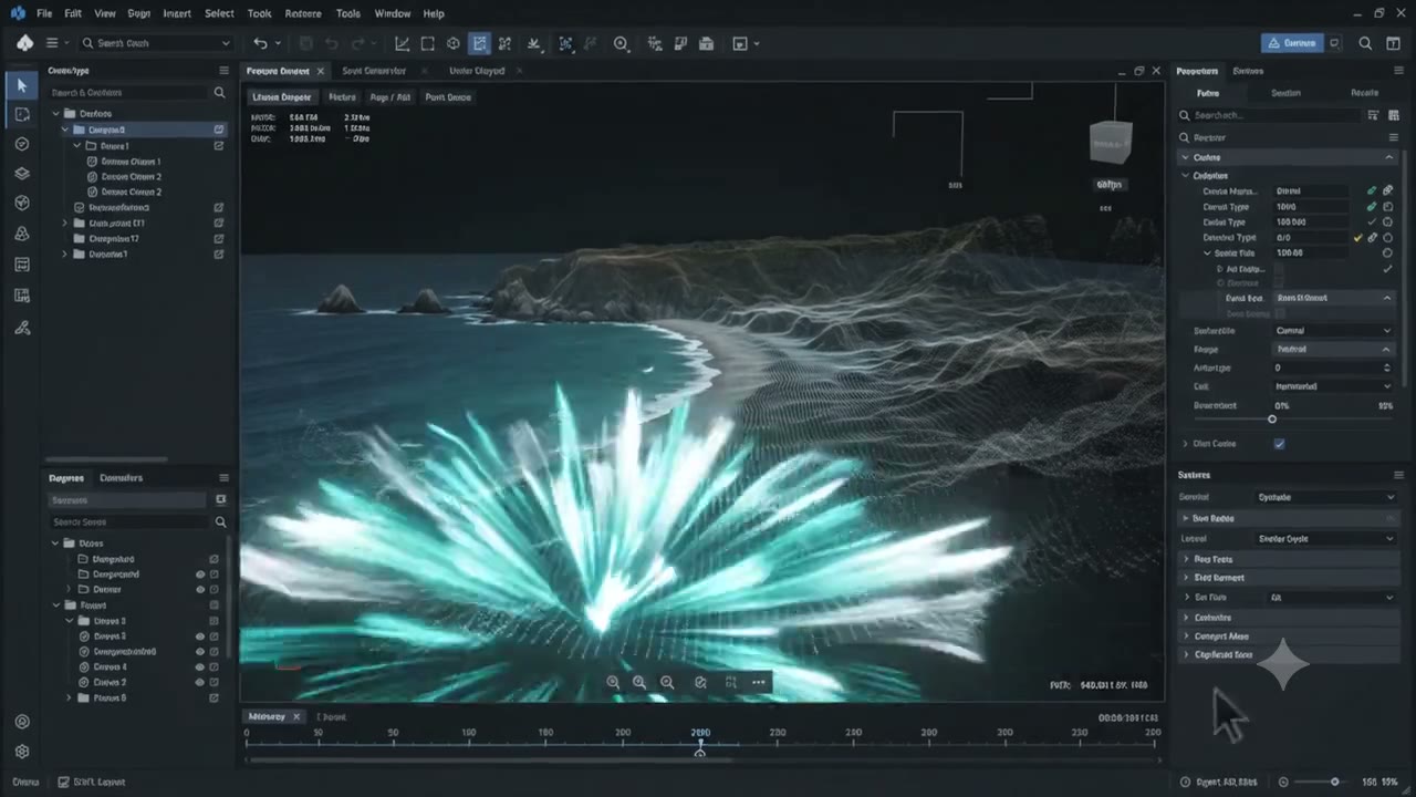
Real projects don't arrive as clean spreadsheets. They arrive as last week's laser scan, a decade of sensor logs, a simulation that ran all weekend, and a folder the client swears is organized. LSD meets your data where it is.
Point clouds & scans
LiDAR, photogrammetry, LAS/LAZ.
Rasters & imagery
GeoTIFF, satellite, drone, instrument imagery.
Meshes, CAD & models
Surfaces, solids, BIM/IFC.
Tables & databases
CSV, SQL, Parquet, and yes, the client's Excel.
Time series & telemetry
Sensors, instruments, monitoring feeds.
Scientific formats
NetCDF, HDF5, simulation outputs.
If it's part of the work, it belongs on the graph.
Shape
Shape. Where the thinking happens.
Shaping is the real work — and the part that usually disappears into scripts nobody can read a year later. In LSD, every method is a node on a shared graph: visible, reusable, explainable. Change one step and only what's downstream reruns; every result is cached, every decision is on record.
Every discipline brings its own verbs — the geophysicist's filters, the structural engineer's load cases, the environmental scientist's models, the data scientist's networks. In LSD, they all speak the same grammar.
Shaping is a team sport. Colleagues join the same graph with live cursors and comments — the engineer, the scientist, and the analyst finally looking at the same thing instead of emailing exports at each other.
And agents are teammates here too. An agent can load data, propose shaping steps, and draft outputs — but every action lands as a visible node in a pending state. Review it, edit it, approve it, or throw it out. Nothing runs behind your back.
Other tools give you an AI in a sidebar. LSD gives your agent a seat at the graph — under the same visibility rules as everyone else.
Shared workspace · live cursors · pending agent nodesreplace with screenshot · 1600 × 1000
Deliver
Deliver. Work that speaks for itself.
The last mile is where reputations are made. Don't hand over a static PDF and hope — deliver results clients can explore.
Interactive charts
Publication-quality, live-linked to the pipeline.
Reports & documents
Assembled from the graph, not copy-pasted at midnight.
Interactive 3D scenes
Let clients orbit the model, not squint at screenshots.
Map navigators
Spatial results your client can pan, zoom, and question.
Dashboards
Living views for long-running projects.
Clean exports
Straight into whatever tool comes next.
Send clients something they can fly through, not flip through.
And when the client asks for next month's update: one click. Same pipeline, new data, same quality. That's what "professional" means here.
Platform
Your methods, as tools. Your tools, as a platform.
Every team has hard-won methods trapped in scripts on one person's laptop. In LSD you wrap them once — Python SDK, hot reload while you build — and they become drag-and-drop nodes anyone can use.
Keep them private to your firm, or publish to the Tool Store and put your specialty in front of every engineer and scientist on the platform.
Every tool published to the store is a new verb — for every human and every agent on the platform. That's how LSD compounds: the more the community builds, the more everyone's pipelines can do.
from lsdtools importshape@shapedefnormalize(inputs):
t = inputs.main
return t.normalize() # edit live, save → re-runs
Trust
Runs where the work lives
LSD is a desktop app on purpose. Client data comes with NDAs, field sites come with no bandwidth — so your models, scans, and datasets stay on your machine unless you decide otherwise. Work offline, sync when you're back. Smart caching keeps multi-gigabyte datasets responsive instead of re-crunching on every change.
Every step visible and auditable — the pipeline is the documentation
Agent actions require approval before they run
Reproducible by construction: same inputs, same outputs, every time
Local-first: no forced cloud, no client data leaving your machine
Tour
See LSD in two minutes
A short walkthrough — bring a dataset, transform it live with your team, and deliver a result.
2-minute product tourreplace with video / poster · 1920 × 1080